
Have you ever felt baffled by those mysterious dollar signs in Excel formulas? You’re not alone! Many Excel beginners, perhaps like yourself, often overlook the significance of these symbols.
But here’s a little secret: mastering dollar signs is a game-changer for anyone aspiring to become a proficient Excel analyst or create powerful Excel tools. Fear not – it’s far simpler than it seems!
In this post, I’ll demystify the use of dollar signs, guiding you step-by-step through their purpose and application. Let’s embark on this journey together and transform confusion into clarity.
Table of Contents
- What Are the Dollar Signs in Excel Formula?
- Why Use the Dollar signs in Excel?
- Understanding Relative Referencing in Excel
- Understanding Absolute Referencing in Excel
- An Example Using Referencing
- Additional Tips for using Dollar Signs in Excel?
- Summary
What Are the Dollar Signs in Excel Formula?
If you see a formula that looks something like:
- =B3 * $A$1
This is an example of using Dollar signs in Excel formula.
Why Use the Dollar signs in Excel?
The Dollar signs are used for indicating Absolute References. Now that statement might not be too helpful but to understand what I mean there are two ways you can reference a cell location in Excel:
- Using a Relative Reference (no Dollar signs)
- Using an Absolute Reference (Dollar signs involved).
Understanding Relative Referencing in Excel
Relative referencing might sound technical, but it’s actually Excel’s default way of handling formulas, and you’ve likely used it without even realizing. Let’s say you’ve made a basic Excel formula before. If you’ve included a cell reference like A1 without any dollar signs, congratulations, you’ve used relative referencing!
So, what is relative referencing? Simply put, it’s how Excel knows what your formula means and applies it to other cells when you drag or copy your formula. It’s like Excel’s way of keeping things in context.
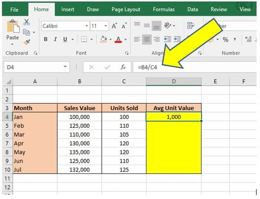
Let’s look at a practical example. Imagine you want to calculate the ‘Average Unit Value‘ in column D. This requires dividing the ‘Sales Value‘ in column B by the ‘Units Sold‘ in column C.
You could type a straightforward equation in cell D4, like =100,000/1,000, but this won’t work well if you drag it down to cell D5. You’d end up having to write out the formula for every cell in Column D, which is a hassle.
Here’s where relative referencing comes in handy.
It tells Excel to divide the cell two columns to the left (column B) by the cell one column to the left (column C). So, for cell D4, the formula becomes =B4/C4.
This way, Excel automatically adjusts the formula for each cell in the column, saving you time and effort.
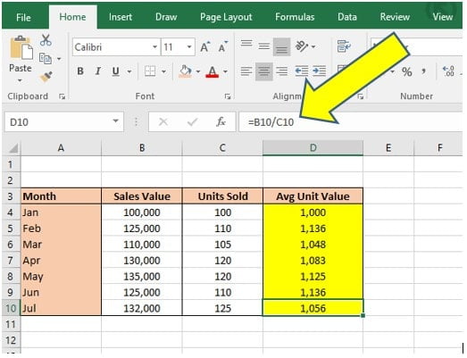
By using the Relative Reference system it will allow you to drag the formula down and apply it to February, March, April and so on without having to enter a new formula every time.
Dragging the formula you created in cell D4 down to cell D10, Excel auto-calculates the correct Average Unit Value for every month. When you look at the formula in cell D10 it has automatically changed to =B10/C10.
Note: this is still saying take the cell 2 Columns to the left and Divide it by the cell 1 Column to the left.
As mentioned previously Relative References are commonly used and most of you will be using them without even realizing what they are. However, there are times when you need to fix the cell location in some way and this is where Absolute Referencing comes in and our Dollar signs.
Understanding Absolute Referencing in Excel
Absolute referencing in Excel is where the dollar signs ($) come into play in your formulas. These dollar signs are crucial; they lock a specific part of your cell reference, ensuring it stays constant when you drag or copy your formula elsewhere.
Now, there are three main ways you can use these dollar signs to anchor your cell references:
- Fixing the Column Position: By placing a dollar sign before the column letter, you fix the column. For example, in =$A1, the ‘A‘ column is fixed. No matter where you drag this formula on your worksheet, it will always refer back to column A, although the row number can change.
- Fixing the Row Position: Here, the dollar sign precedes the row number, fixing the row. In =A$1, the 1st row is fixed. So, if you move this formula around your worksheet, it will always point back to row 1, but the column can vary.
- Fixing Both Column and Row: When you want to anchor a specific cell entirely, you put dollar signs in front of both the column letter and row number, like in =$A$1. This locks cell A1, meaning no matter where you copy or drag the formula, it will always reference cell A1.
Understanding these three methods of using dollar signs for absolute referencing in Excel empowers you to control exactly how your formulas behave when moved or copied, giving you precision and consistency in your data management tasks.
An Example Using Referencing
Referring back to the previous Example imagine if you now have a Sales Commission of 10% that your boss wants included in the table.
You could use a formula that multiplies the Sales Value by the value of 10% but what if your boss then tells you the Commission rate was wrong or needs to be changed? It would mean you need to change all the formulas in every cell again and that is not very efficient.
Instead you can use Absolute Referencing to set a Commission % cell and then always refer to that cell in your formula.
By doing this if you want to change the Commission to a hefty 20% and see how it affects the numbers you only need to change one value in the Commission % cell and all the totals will recalculate:
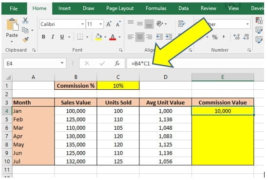
In the image above the ‘Commission %‘ cell is in cell C10 and it has been set to 10%.
In the ‘Commission Value‘ column of the table (Column E) the first formula is entered to cell E4 which is =B4*C1.
Remember that to Excel the underlying meaning of this formula is take the cell 3 columns to the left(B4) and multiply it by the cell 2 Columns to the left and 3 Rows up (C1). If you leave this formula as it is watch what happens when it is dragged down to E10:
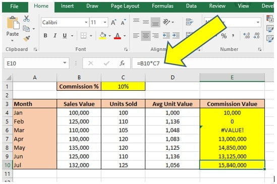
As you can see the formula starts fine in cell E4 but as soon as you drag the formula down the other months it goes horribly wrong. To see the problem you only need to look in cell E10 which shows the formula to be = B10 * C7.
This is clearly not what was intended as while B10 is the correct Sales Value to use C7 is the Units Sold in May and not the Commission percentage.
What Did We Do Wrong?
We forgot to set the Absolute Reference.
Excel is doing its job, remember Excel thinks it should be multiplying the cell 3 Columns to the left by the cell 2 Columns to the left and 3 Rows up…if you do a quick zoom around the table that is working so it’s not Excels fault, the fault is with us.
What we need to do is change the underlying meaning to Excel by saying Multiply the cell 3 columns to the left by the cell C1 and always the cell C1 as that is the Commission %.

You can see from the above image the formula in cell E4 now reads = B4 * $C$1.
Referring back remember that a Dollar sign before the Column location and before the cell location is the same as making a specific cell a fixed-point.
By including the Dollar sign before the Column letter C and before the Row number 1 the cell C1 becomes a fixed-point and the underlying meaning is changed to multiply the cell 3 Columns to the left by the value in C1, drag that version down the table and see the results:

The formula has now worked as planned. A quick check again in cell E10 shows that the formula is multiplying B10 (the cell 3 columns to the left) by C1, perfect!
Additional Tips for using Dollar Signs in Excel?
To use Absolute References in Excel formula you can manually type the Dollar signs around the cell location or you can simply toggle the 3 Absolute Reference options using the shortcut key of F4.
To use the Shortcut key make sure the cursor is directly to the left of your cell reference, i.e. if you want to add absolute references to = 50 * A1 then make sure the cursor is flashing to the left of A, then hit F4. Hit F4 once and it will turn it into a fixed cell location, hit F4 again and it will change to just a fixed row location and finally hit F4 a third time if you want just the column to be fixed.
Summary
This guide aimed to clarify the use of dollar signs in Excel formulas, a crucial technique often overlooked by beginners.
Understanding this concept is essential for your Excel learning journey, as it forms the foundation of creating absolute references in formulas.
This knowledge is not only vital for current tasks but also pivotal for advanced Excel operations. It’s a fundamental skill that enhances your overall Excel proficiency, ensuring accuracy and efficiency in your data management.
Keep Excelling,

Now that you understand the significance of dollar signs in Excel, expand your Excel expertise further by learning how to count in Excel. Whether it’s values, text, or blanks, our guide on “How to Count in Excel: Values, Text, and Blanks” offers insightful techniques to enhance your data analysis skills.