
How To Multiply in Excel Like a Pro: A Step-by-Step Guide
For small and midsize companies, Microsoft Excel is often the default spreadsheet tool when working with numbers in any context.
Excel's versatility makes it suitable for all calculations, but it also offers numerous ways to accomplish any given task. For example, there are many ways to multiply using Excel. If you've ever wondered how to multiply in Excel, here is a step-by-step guide to multiplying numbers, cells, columns, and more.
Multiplying numbers in Excel
Multiplication in Excel can happen with a simple formula or via more complex methods, such as the PRODUCT function. Here are some examples:
How to multiply two numbers in Excel
The easiest way to multiply using Excel is with two numbers in a single cell.
For instance, if you want to multiply 2 times 4, open Excel and click on any blank cell. Type an equal sign and then the two numbers you want to multiple, so =2*4. (The asterisk between the two numbers is the Excel multiply symbol.)
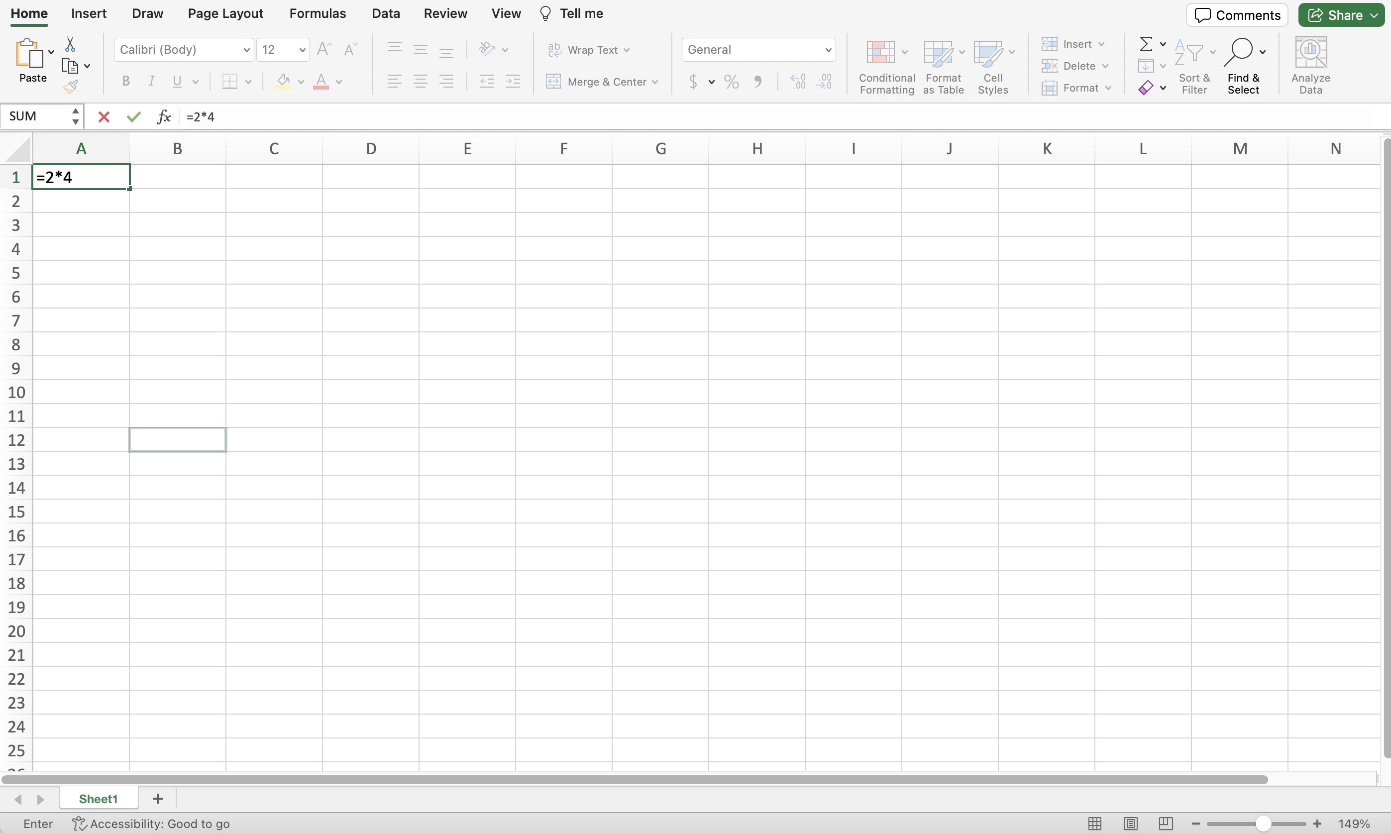
All screenshots were captured by the author on Microsoft Excel 365 on macOS 14.1, 2023.
Now press "Return" or "Enter" to complete the calculation. The value in the cell is now 8, which is the result of 2 times 4.
How to multiply a range of numbers in Excel
While the single-cell Excel multiplication formula is quick and easy, you'll likely want to multiply numbers already appearing in different cells. Rather than typing out those numbers, use Excel's PRODUCT function to multiply a range of numbers.
How to use the PRODUCT function in Excel
Excel's PRODUCT function lets you specify which cells contain the numbers you want to multiply.
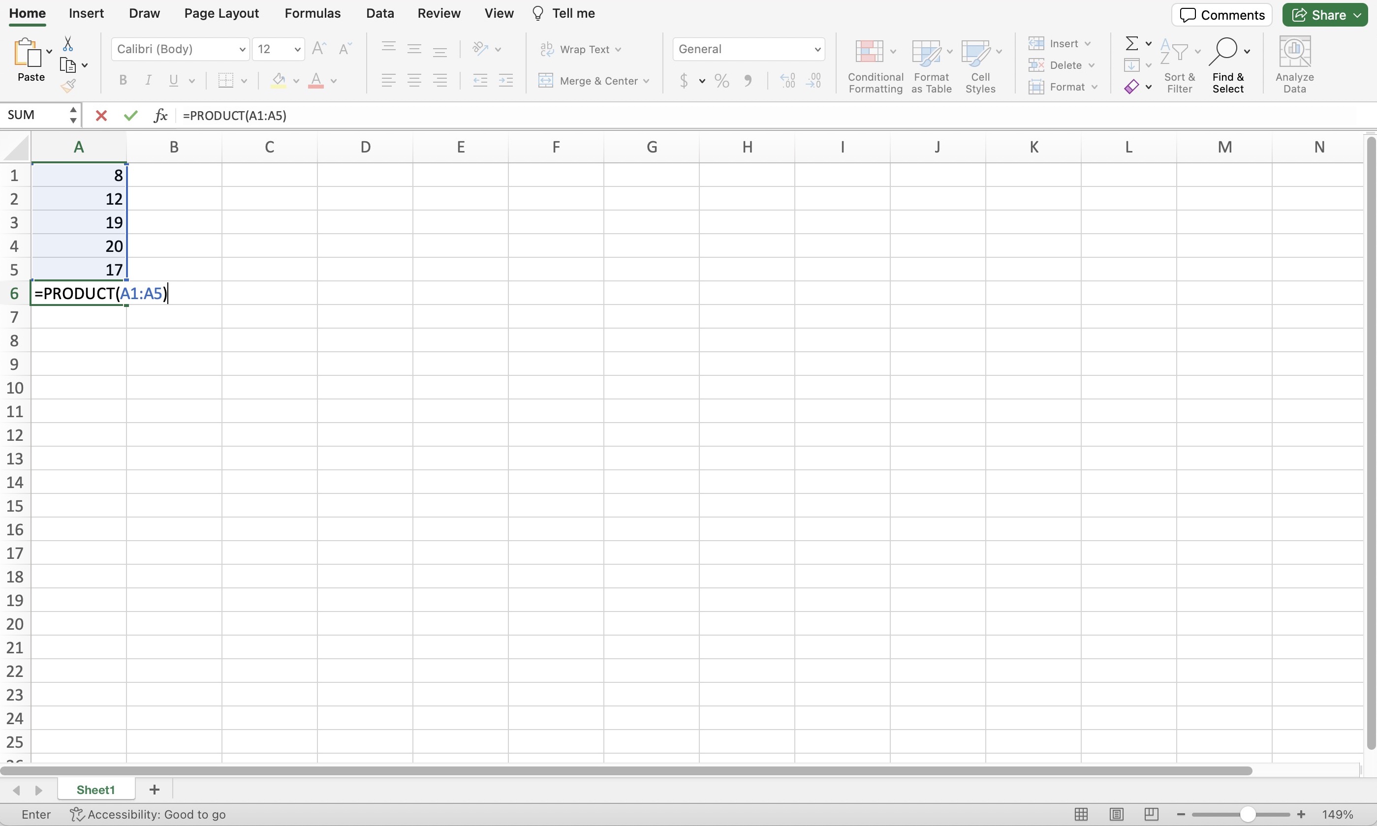
In this example, cells A1 through A5 contain different numbers. To multiply this range of cells, click on a blank cell (A6 in this example) and enter the formula =PRODUCT(A1:A5).
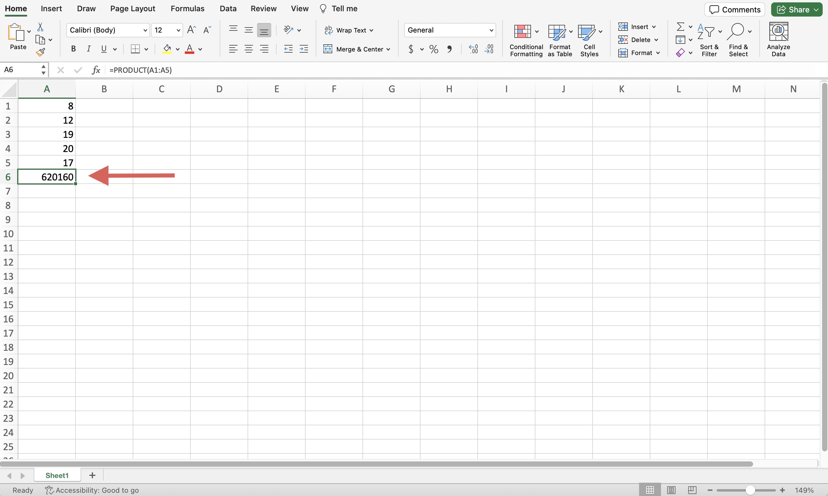
Press "Return" or "Enter." The result of this calculation appears in cell A6.
Multiplying cells in Excel
Multiplying cells in Excel is much the same as multiplying numbers. Instead of entering numbers into the formula, you use cell names, as in these examples:
How to multiply two cells in Excel
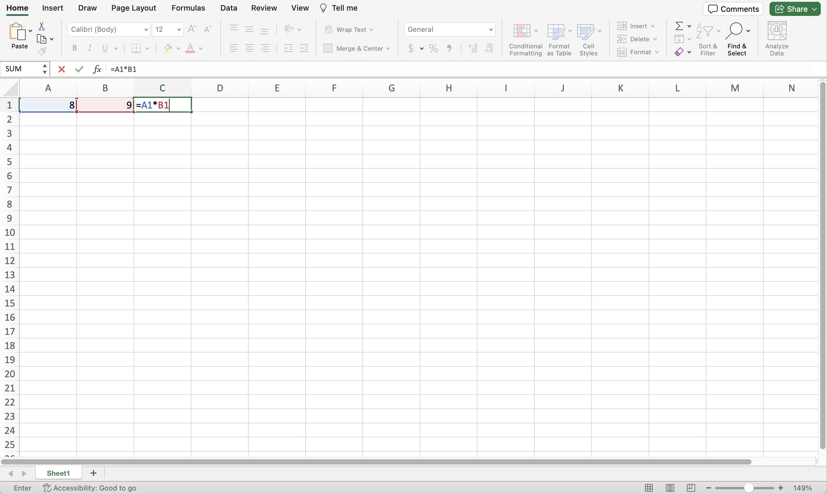
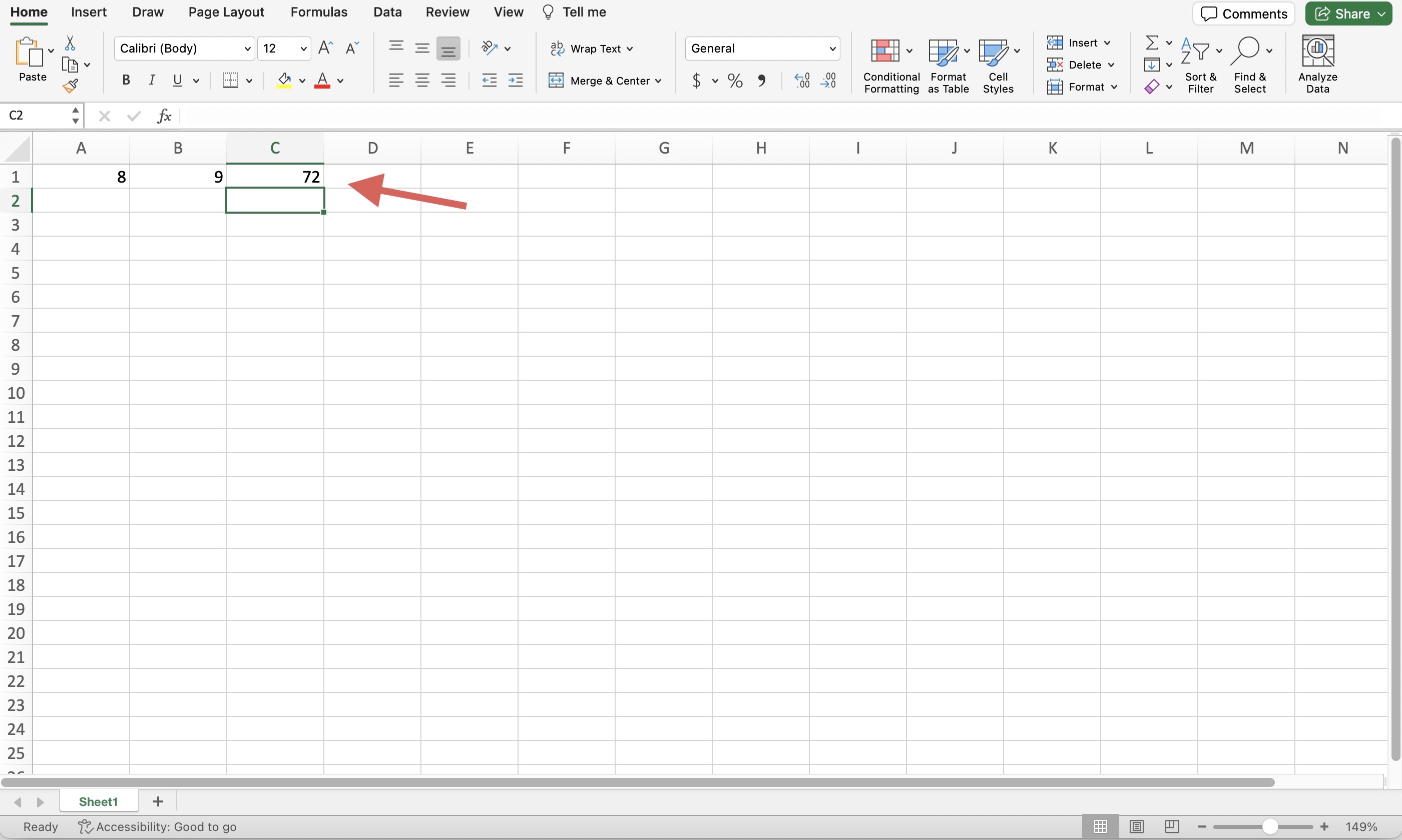
In this spreadsheet, cell A1 contains the number 8, and cell B1 has a 9. To multiply these two cells, click on a blank cell and type the equal sign and then the range, so =A1*B1.
Now press "Return" or "Enter"; the result of multiplying the two cells appears.
What is the difference between multiplying numbers and multiplying cells in Excel?
Multiplying numbers and multiplying cells in Excel work essentially the same way. The main difference is that when you multiply cells in Excel, you type the cell name into the formula rather than a number. Otherwise, the same formulas for multiplying numbers can work to multiply cells in Excel.
Multiplying columns in Excel
You can also multiply entire columns using the Excel multiplication formula.
To start this type of calculation, click on a blank cell and type the equal sign. Next, type the range of cells in the first column, using a colon between the beginning and end of the range.
In this example, the first column is the range of cells from A1 to A4. You will type the range as A1:A4. Now, type an asterisk followed by the range of the second column (B1:B4 in this case). So, our calculation looks like =A1:A4*B1*B4.
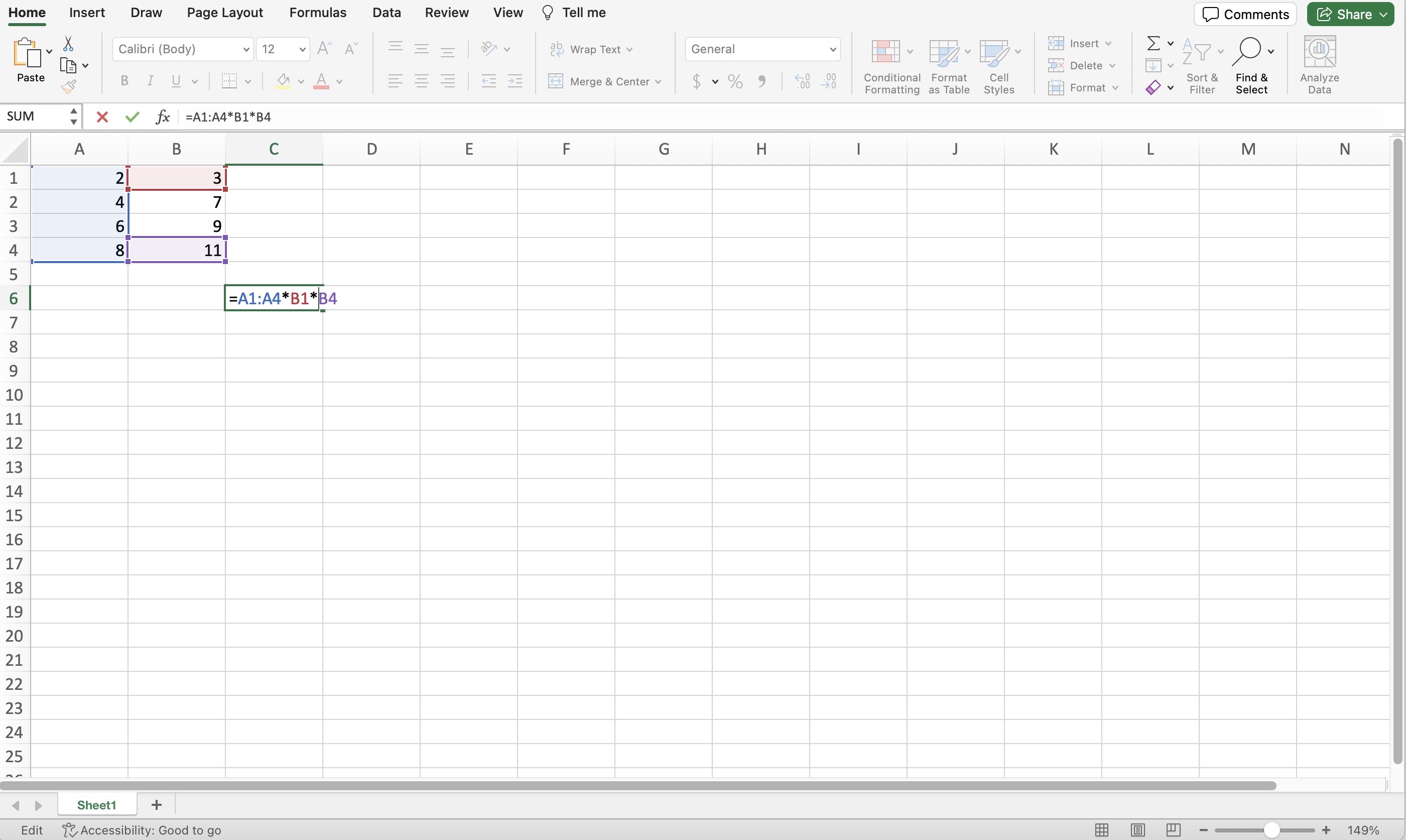
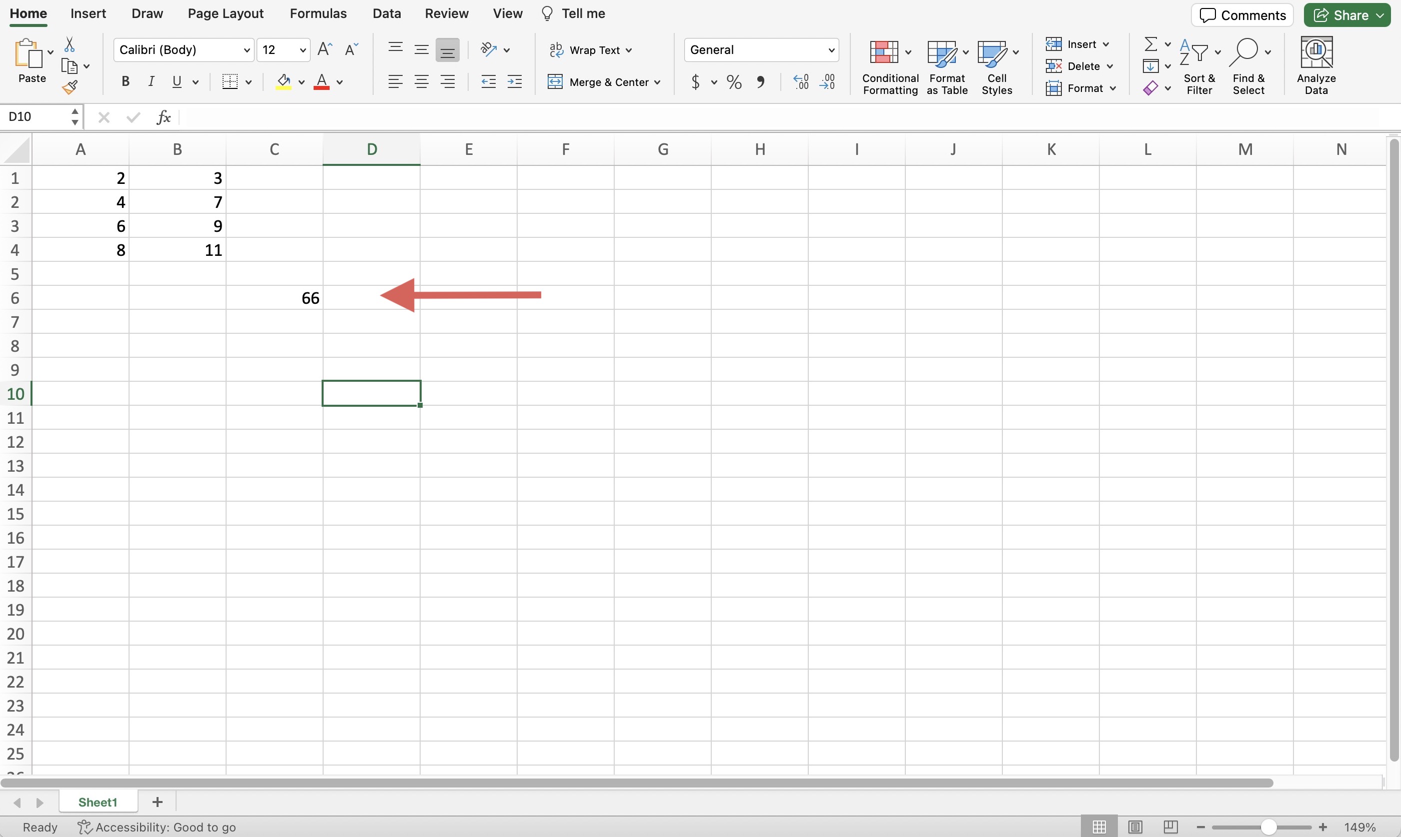
Now press "Ctrl+Shift+Enter" (or "Ctrl+Shift+Return" on a Mac). This prompts Excel to wrap the formula in curly braces and perform the calculation. Now, you will see the result, which is the sum of the first column multiplied by the sum of the second column.
How to multiply by percentage in Excel
To multiply by a percentage in Excel, use the standard multiplication formula with a percentage figure. For instance, typing =50*10% and pressing "Return" or "Enter" in a blank cell will return the result, which is 5.
You can also use cells instead of numbers to multiply by percentages. For example, typing =A2*B2 will multiply the values contained in cells A2 and B2.
Multiplication in array formulas
Excel supports more complex multiplication functions. This includes arrays, which are groups of numbers organized in columns and rows. The MMULT function allows you to multiply two arrays using the matrix multiplication method. This is where the first row of one array is multiplied by the first column of the second array.
In this example, the first array has three columns and two rows, while the second array has two columns and three rows.
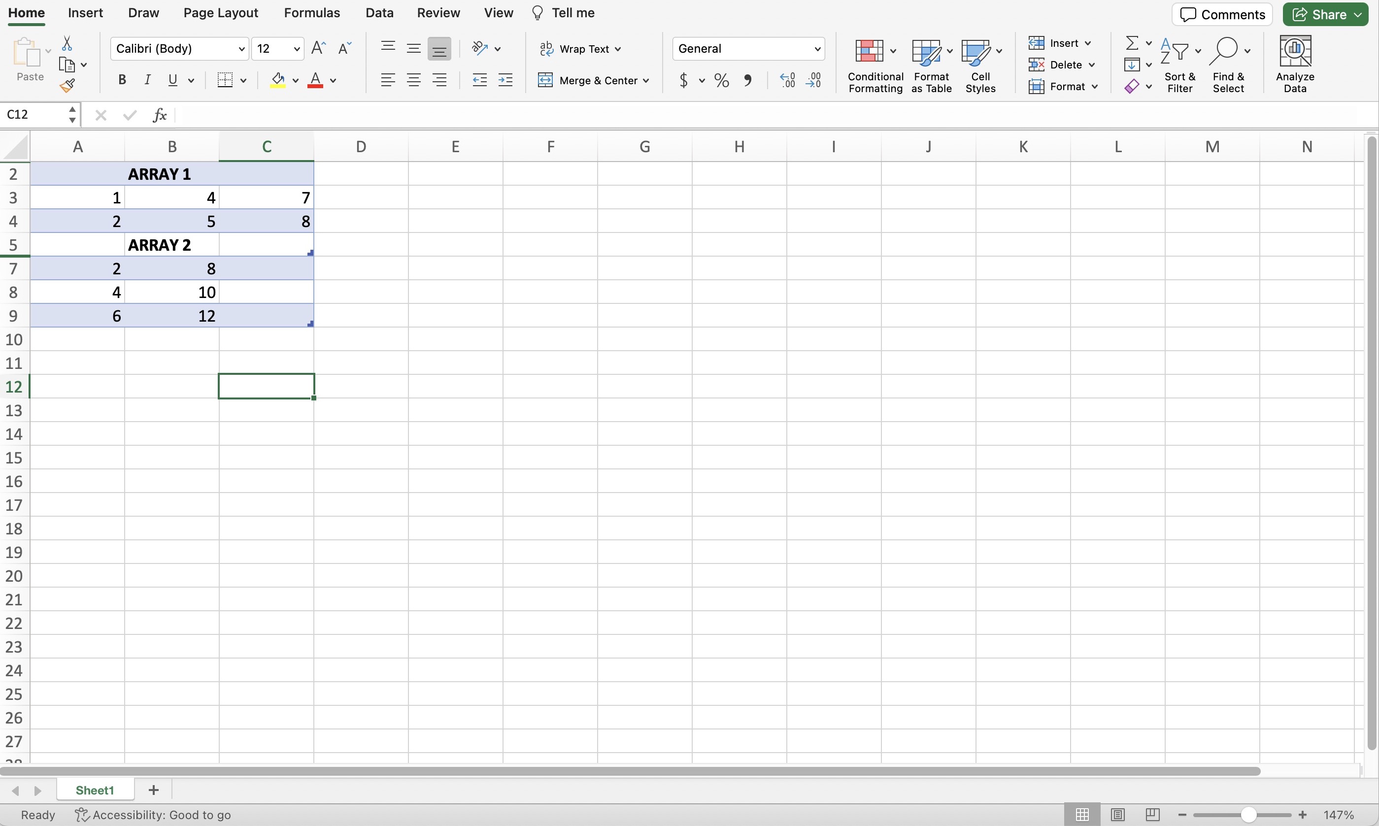
You can use the MMULT function to multiply the two rows of the first array by the two columns, with the results in a new array of two rows and two columns. The syntax looks like this =MMULT(array1,array2).
To use the cell ranges in the example arrays shown here, the formula is =MMULT(A3:C4,A7:B9).
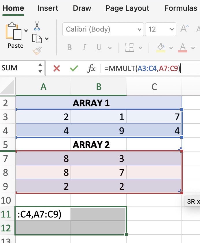
Press "Ctrl+Shift+Enter" or "Ctrl+Shift+Return" to calculate the result.
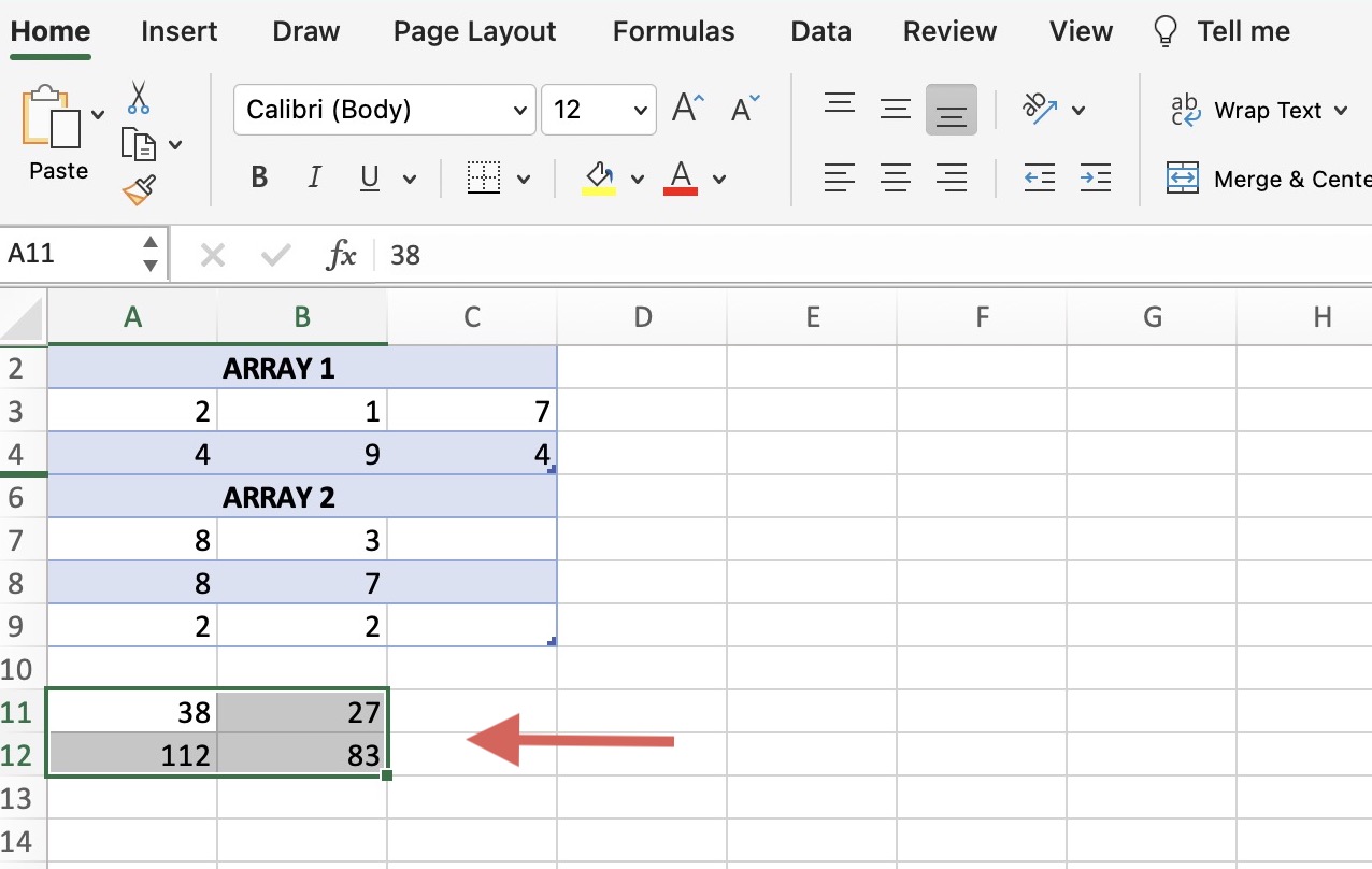
Here’s a quick look at how MMULT used matrix multiplication to arrive at these results:
The first row values of Array 1 are 2, 1, and 7, and the first column values of Array 2 are 8, 8, and 2.
The first value of the results array is 38, which was calculated like this:
=(2 * 8) + (1 * 8) + (7 * 2)
=16 + 8 + 14
= 38
MMULT then repeats the same matrix multiplication formula for the other rows and columns.
How to multiply and sum in Excel
The SUMPRODUCT function in Excel sums the results of multiple arrays. The syntax for this function is =SUMPRODUCT(array1,array2). You can add as many arrays as you like to the SUMPRODUCT formula.
Common Excel multiplication formulas
While SUMPRODUCT and MMULT are the more advanced multiplication formulas in Excel, the two most common formulas work fine for most situations:
Multiply two numbers or cells with an asterisk, as in =4*3 or =A2*B3
Use the PRODUCT function to quickly multiply a range, such as =PRODUCT(F1:F10)
Use PRODUCT for any combination of numbers, cells, and ranges, such as =PRODUCT(F1:F10,G3:G5)
Common Excel multiplication mistakes
Most multiplication errors stem from incorrect formula syntax or using a symbol other than the asterisk for simple multiplications. When multiplying ranges, ensure that all cell references are correct. Mistyping a cell range could lead to an error.
Excel makes multiplication quick and easy
As an accounting and finance tool, Excel is invaluable for many small and midsize businesses. Excel's versatility allows you to work at whatever level you're comfortable, but learning the common multiplication formulas can speed up your team's workflows.
Check out more Software Advice resources on accounting and data tools: